Discounted cash flow (DCF) is a core financial valuation method used to estimate the current worth of an investment, company, or asset based on its projected future cash flows. It incorporates the principle of the time value of money, recognizing that a dollar received today is worth more than a dollar received in the future. In Canada, DCF analysis is widely applied by investors, corporate managers, and analysts to value stocks, assess real estate projects, make capital budgeting decisions, and determine the intrinsic value of businesses. Understanding DCF is essential for anyone involved in investment finance or corporate financial management, as it provides a fundamental, cash-flow-based approach to valuation that goes beyond simple market prices.
What Is Discounted Cash Flow Analysis
Discounted cash flow analysis is a valuation method that estimates what an investment or business is worth today by projecting its future cash flows and discounting each one back to its present value. The core idea is that the value of any asset is fundamentally the sum of all the cash it will generate for its owners in the future, adjusted for the fact that money available now is more valuable than the same amount in the future. This adjustment is done using a discount rate, which captures both the time value of money and the risk that those future cash flows may not materialize as expected. DCF is one of the main approaches in formal company and project valuation and is often cross-checked against simpler market-based methods. The method is applicable to a wide range of valuation scenarios, including investment finance, real estate development, corporate financial management, actuarial science, and patent valuation.
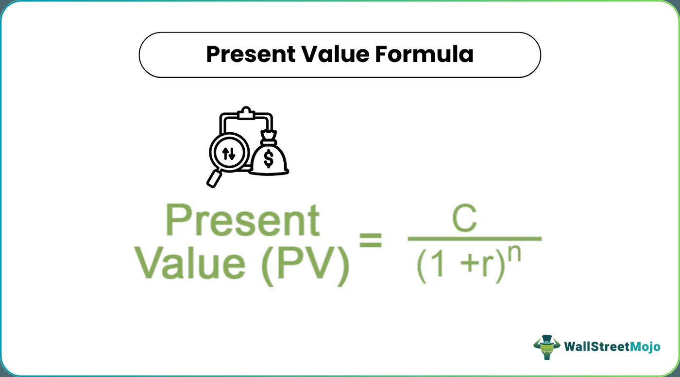
The Mathematics and Formula of DCF
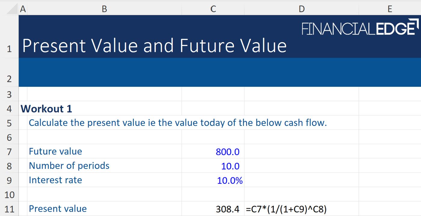
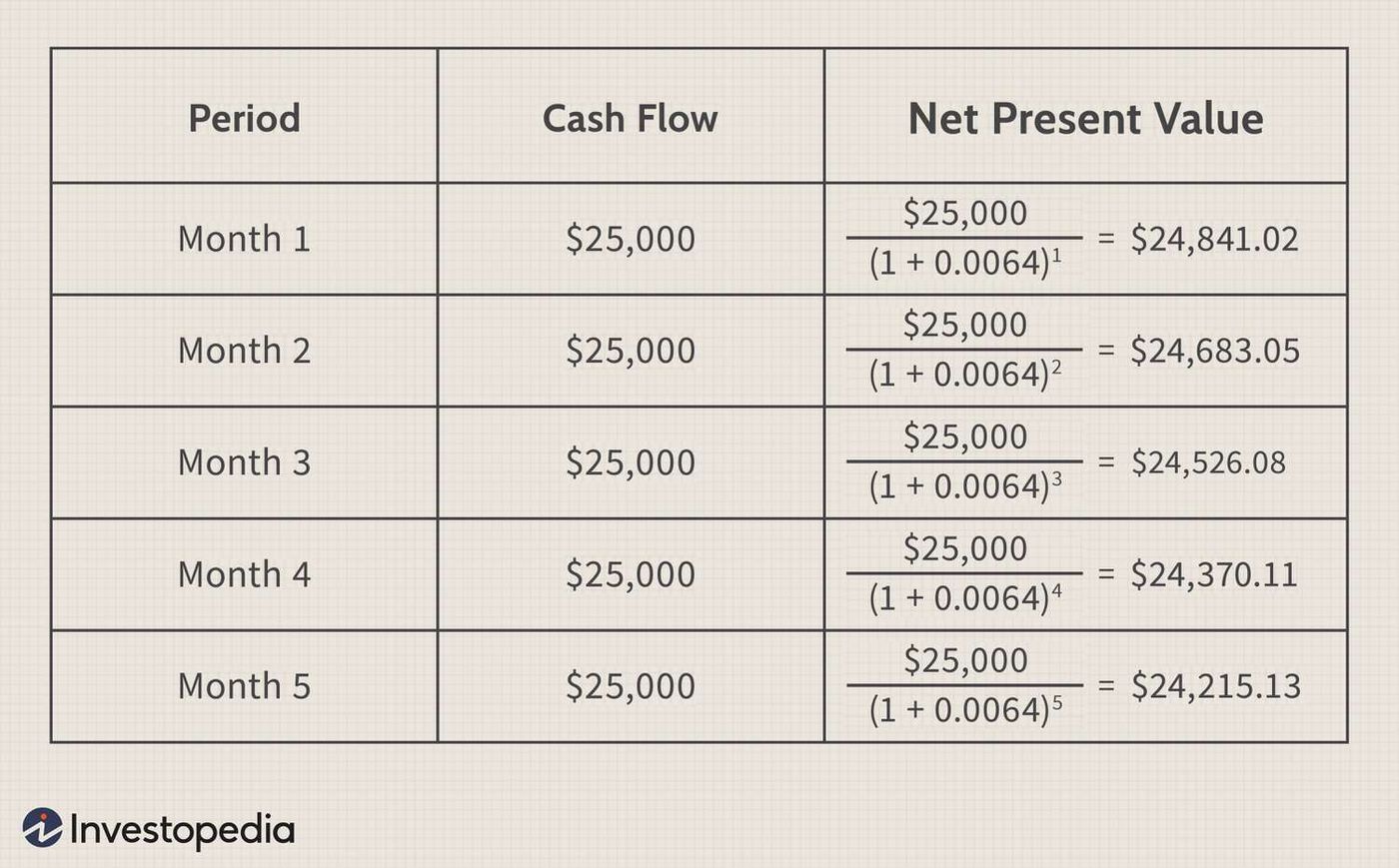
The mathematical foundation of DCF is derived from the present value formula for calculating the time value of money. The basic formula discounts a single future cash flow back to the present. For multiple cash flows over different time periods, the discounted present value is the sum of each individual discounted cash flow. This sum is the net present value (NPV), which serves as the estimated value of the cash flow stream. The formula assumes a constant discount rate throughout the forecast period. When the cash flow stream is assumed to continue indefinitely beyond a discrete forecast period, a terminal value is calculated and added to the NPV of the finite forecast. For continuous cash flows, the summation in the standard formula is replaced by an integration. The formula for the discounted present value of a series of cash flows is the sum of each future cash flow divided by one plus the discount rate raised to the power of the time period. The internal rate of return can be solved for if the present value and all future cash flows are known, representing the discount rate that makes the net present value equal to zero.
Determining the Discount Rate
The discount rate is a critical input in DCF analysis, representing the required rate of return for the investment. It answers the question of how much money would have to be invested currently, at a given rate of return, to yield the forecast cash flow at its future date. This required return incorporates two main components. The first is the time value of money, represented by a risk-free rate such as the yield on government bonds, which compensates investors for the delay in receiving cash. The second is a risk premium, which reflects the extra return demanded for the risk that the cash flow might not materialize. For valuing equity, the required return is often determined using the Capital Asset Pricing Model (CAPM), which calculates the cost of equity as the risk-free rate plus a beta coefficient multiplied by the equity risk premium. For valuing an entire firm or project, the discount rate is typically the Weighted Average Cost of Capital (WACC), which blends the cost of equity and the after-tax cost of debt, weighted by their proportions in the company's capital structure. Other models exist but are less common in industry practice compared to exponential discounting. An alternate, although less common approach, is to apply a fundamental valuation method such as the T-model, which relies on accounting information.
Common DCF Valuation Approaches
Several distinct DCF methods are used for valuation purposes, with the choice depending largely on the capital structure and the perspective of the valuation. The assumptions used, especially the discount rate and cash flow projections, are as important as the precise model chosen. The primary methods include the flows to equity approach, the adjusted present value approach, the weighted average cost of capital approach, and the total cash flow approach. Each method uses a different income stream and corresponding discount rate to arrive at a value. The flows to equity approach discounts the cash flows available to the holders of equity capital, after allowing for the cost of servicing debt capital, which makes explicit allowance for the cost of debt but requires judgement on the choice of discount rate. The adjusted present value approach discounts the cash flows before allowing for debt capital but adds the value of tax relief on debt interest, which is simpler for projects without earmarked debt finance but also requires discount rate judgement. The weighted average cost of capital approach uses the WACC to discount the unlevered free cash flows from the project, overcoming the need for debt to be earmarked to specific projects. The total cash flow approach discounts the total cash flows to the firm with the tax shield on debt interest included in the cash flows rather than the discount rate. This distinction shows DCF can value various ownership interests, including equity or debt holders, or the company based on total invested capital.
Practical Application and Steps in Canada
In Canadian finance, applying DCF analysis involves a detailed, step-by-step process to estimate a company's intrinsic value or an investment's worth. The process begins with projecting free cash flows, which requires estimating future revenue, expenses, taxes, capital expenditures, and changes in working capital over a typical forecast window of five to ten years. These projections should be based on historical trends, realistic growth assumptions, and industry benchmarks to avoid over- or underestimation. The next step is determining a terminal value at the end of the forecast period, often using the Gordon Growth Model for mature businesses or an exit multiple method for others. A discount rate, such as WACC tailored to the company's risk profile, is then applied to discount all projected cash flows and the terminal value back to their present value. The sum of these present values is the enterprise value. To find an equity value per share, net debt is subtracted from the enterprise value and the result is divided by the number of shares outstanding. This intrinsic value per share can then be compared to the current market price to identify potential investment opportunities. DCF analysis is only as reliable as its inputs, which is why Canadian investors dedicate serious time to ensuring forecasts are as fact-based as possible. Using an online DCF calculator or spreadsheet template can help input variables for quick analysis, but understanding the underlying assumptions remains crucial for interpreting results.
The step-by-step calculation of discounted cash flow involves estimating all future cash flows and discounting them using a cost of capital to give their present values. This process sums all future cash flows, both incoming and outgoing, to arrive at a net present value figure. The calculation is mathematically expressed by the discounted cash flow formula, which sums the present values of individual cash flows. This method is foundational to the DCF analysis used in investment finance and corporate financial management.
- Project the free cash flow a business is expected to generate in the coming years, using the formula: FCFF = EBIT × (1, tax rate) + non-cash charges, CapEx, change in working capital.
- Determine the terminal value using either the Gordon Growth Model (Terminal Value = [FCFFₙ × (1 + g)] / (r, g)) for stable businesses or the Exit Multiple Method for transitional businesses.
- Apply the discount rate to the projected cash flows and terminal value to calculate their present value, often breaking it down year by year for sensitivity analysis.
- Calculate the enterprise value by summing the present value of projected cash flows and the present value of the terminal value.
- Subtract the company’s net debt (total debt minus cash) from the enterprise value.
- Divide the resulting equity value by the number of shares outstanding to determine the intrinsic value per share.
Completing the DCF calculation provides a net present value which serves as a valuation metric for a security, project, company, or asset. This net present value can be compared to a market price to inform investment decisions. The process can also be reversed, using cash flows and a present value to solve for the discount rate, which is used in bond markets to obtain the yield. This linkage makes DCF analysis a core tool for valuation in finance.
Limitations and Criticisms of DCF
Despite its theoretical soundness, DCF analysis faces significant practical limitations and criticisms. The primary difficulty is the reliability of forecasts, as the model assumes an ability to accurately predict revenue and earnings several years into the future. Studies have shown that growth is neither predictable nor persistent, a problem rooted in the philosophical issue of induction, where past performance does not guarantee future results. This makes DCF models especially challenging for unpredictable industries or companies without a steady cash flow history. For example, in commercial real estate, DCF models can be problematic because discount rate assumptions may not persist, and historic rent increases may not account for the cyclical nature of the market, potentially leading to overvaluation during boom periods. For early-stage technology companies or startups, the lack of historical data and high uncertainty about future development factors make DCF models particularly difficult and reliant on a range of scenario analyses. The terminal value often constitutes a large portion of the total calculated value and is highly sensitive to assumptions about long-term growth and discount rates, which can significantly sway the final valuation. The U.S. Securities and Exchange Commission mandates that mutual funds warn investors that past returns are not indicative of future results, a principle that directly challenges the forecasting foundation of DCF. In mining or healthcare settings, industry-specific risks may require modified discount rate formulae, as risk characteristics can differ dramatically by property or project.
The shortcomings of DCF are evident in its reliance on forecasting future cash flows and growth rates, which studies show are neither predictable nor persistent. This forecasting difficulty is problematic due to the problem of induction, which assumes future events will follow past patterns. The terminal value, which often represents a large share of total value, is highly sensitive to growth and discount rate assumptions. These issues can be particularly pronounced in industries with volatile or unpredictable cash flows.
- Real Estate: Reliance on current market discount rates and historic rent increases often fails to factor in the cyclical nature of markets, leading to potential overvaluation when loans are made during booms.
- Early-stage Technology Companies: A lack of historical data and high uncertainty about future cost of capital, growth rates, and cash flows make forecasts lack credibility.
- Unpredictable Industries: For sectors where revenue swings wildly, forecasting cash flows three to five years out becomes highly unreliable.
- Over-reliance on Terminal Value: The terminal value often represents a large share of total value, making the entire valuation highly sensitive to assumptions about long-term growth and discount rates.
The limitations of DCF analysis underscore why it is best suited for valuing mature companies in stable sectors. In such environments, future cash flows are more consistent and can be estimated with greater reliability. The method's assumptions about constant growth beyond a forecast period are more tenable when a company operates in a stable industry. This makes DCF a more reliable tool for sectors like utilities compared to highly volatile or growth-oriented industries.
Historical Development of DCF
The concept of discounting future cash flows has ancient roots, dating back to when money was first lent at interest. Its use in industrial analysis is documented as early as 1801 in the UK coal industry. However, DCF analysis gained prominence as a formal valuation method for stocks following the stock market crash of 1929. The method was first formally expressed in modern economic terms by Irving Fisher in his 1930 book The Theory of Interest and by John Burr Williams in his 1938 text The Theory of Investment Value. Throughout the 1960s, discounted cash flow was widely discussed and developed within financial economics. Its adoption expanded into legal and regulatory areas in the 1980s and 1990s, when U.S. courts began employing the concept in valuations. This historical progression established DCF as a fundamental component of modern financial analysis. Discounted cash flow valuation is differentiated from accounting book value, which is based on the historical amount paid for an asset rather than its future income potential.
The evolution of discounted cash flow can be traced from its use in ancient times when money was first lent at interest. It was used in the UK coal industry as early as 1801. Following the stock market crash of 1929, it gained popularity as a stock valuation method. Irving Fisher in 1930 and John Burr Williams in 1938 first formally expressed the DCF method in modern economic terms, leading to its widespread discussion in financial economics in the 1960s.
- Ancient Times: Calculations used in some form since money was first lent at interest.
- 1801: Documented use in the UK coal industry for industrial analysis.
- 1929: Gained popularity as a valuation method for stocks following the market crash.
- 1930: First formal modern economic expression by Irving Fisher in The Theory of Interest.
- 1938: Formal expression by John Burr Williams in The Theory of Investment Value.
- 1960s: Widely discussed and developed within the field of financial economics.
- 1980s and 1990s: U.S. courts began employing the DCF concept in legal valuations.
This progression shows discounted cash flow evolving from a basic concept of lending at interest to a formalized academic and practical tool. It was widely discussed in financial economics in the 1960s, solidifying its theoretical foundation. U.S. courts began employing the concept in the 1980s and 1990s, demonstrating its acceptance in legal valuation contexts. Today, it is widely used in investment finance, real estate development, corporate financial management, actuarial science, and patent valuation.
Key Inputs and Calculation Details
The accuracy of a DCF model hinges on the quality and justification of its key inputs. The most critical input is the projection of free cash flow to the firm, which is calculated as EBIT times one minus the tax rate, plus non-cash charges, minus capital expenditures, minus the change in working capital. Forecasting this requires detailed assumptions about revenue growth, profit margins, tax rates, and reinvestment needs. The discount rate must be carefully selected to match the risk profile, with WACC being the standard for firm valuation. The terminal value calculation is another major input, with the Gordon Growth Model formula being terminal value equals the final year's free cash flow multiplied by one plus the perpetual growth rate, divided by the discount rate minus the growth rate. The exit multiple method applies an industry-specific multiple to a final year financial metric like EBITDA. The forecast period is typically five to ten years, long enough to capture meaningful growth but not so long that assumptions become guesswork. For the valuation of a stock, the final step involves reconciling the enterprise value with market data and subtracting net debt to find equity value. Each of these inputs carries inherent uncertainty, and small changes can produce vastly different valuations, which is why sensitivity analysis is a recommended practice.
Frequently asked questions
What is discounted cash flow used for in Canada?
In Canada, discounted cash flow analysis is widely used by investors, financial analysts, and corporate managers for several key purposes. It is a primary method for valuing publicly traded stocks to determine if they are overvalued or undervalued relative to their intrinsic worth. It is also extensively applied in real estate development to estimate the value of investment properties based on projected rental income and expenses. Furthermore, Canadian companies use DCF for corporate financial management decisions, such as evaluating capital projects, mergers and acquisitions, and capital budgeting for new equipment or facilities.
How do you choose a discount rate for a DCF analysis?
Choosing an appropriate discount rate is a critical and assumption-driven step in DCF analysis. For valuing a company's equity, the discount rate is often the required return on equity, which can be estimated using models like the Capital Asset Pricing Model (CAPM). For valuing an entire firm or project, the most common discount rate is the Weighted Average Cost of Capital (WACC), which blends the cost of equity and the after-tax cost of debt based on the company's capital structure. The rate must reflect the time value of money, typically using a risk-free benchmark like government bond yields, plus a risk premium specific to the investment. The selection requires careful judgment and should align with the risk profile of the cash flows being discounted.
What are the main inputs needed for a DCF model?
Building a DCF model requires several key inputs. The most fundamental is a projection of future free cash flows, which involves forecasting revenue, profit margins, taxes, capital expenditures, and changes in working capital. A second crucial input is the discount rate, such as WACC, which reflects the cost of capital and risk. Third, a forecast period must be defined, typically five to ten years. Fourth, an estimate of terminal value is needed to account for cash flows beyond the explicit forecast horizon, often calculated using a perpetual growth model or exit multiple. Finally, data on the company's capital structure, debt, and number of shares outstanding are required to translate an enterprise value into a per-share equity value.
Why is the terminal value so important in a DCF?
The terminal value frequently represents a very large share of the total value calculated in a DCF model, often more than half. This is because it captures the value of all cash flows expected beyond the explicit forecast period, which for a going concern can extend indefinitely. Consequently, the DCF result is highly sensitive to the assumptions used to calculate terminal value, particularly the long-term growth rate and the discount rate applied. Small changes in these assumptions can lead to significant swings in the final valuation, which is why analysts must use conservative and justifiable estimates to avoid substantial overvaluation or undervaluation.
What types of companies are not suitable for DCF analysis?
DCF analysis is less suitable or more challenging for certain types of companies. Young startups or early-stage technology companies with little to no historical financial data and highly unpredictable future cash flows are poor candidates, as the analysis becomes more guesswork than reliable estimation. Similarly, companies in extremely volatile or cyclical industries where revenue swings wildly from year to year make accurate long-term forecasting nearly impossible. The method is most reliable and commonly applied to mature companies in stable industry sectors, such as utilities or established consumer goods firms, where cash flows are more consistent and predictable.
How does DCF account for risk?
DCF accounts for risk primarily through the discount rate. The discount rate is not just a measure of the time value of money. It also includes a risk premium. This premium compensates the investor for the uncertainty that the projected cash flows may not be received in full or on time. A higher perceived risk leads to a higher discount rate, which in turn reduces the present value of future cash flows. The risk premium can be derived from models like CAPM, which considers the asset's sensitivity to overall market movements. Therefore, riskier investments are penalized with a higher hurdle rate, ensuring that the valuation reflects the likelihood of the cash flows materializing.
Sources and further reading
- Discounted cash flow (Wikipedia) en.wikipedia.org
- Discounted Cash Flow (DCF), Canadian Accounting Glossary rncanada.ca
- DCF analysis: how to estimate a stock's value wealthsimple.com
- Discounted Cash Flow Calculator for Businesses venn.ca
- Discounted Cash Flow (DCF) analysis moomoo.com
This article explains how things work and is not financial, tax or legal advice. Rules, limits and rates change, so check the current figures with the Canada Revenue Agency, your province or your financial institution before you act.